Software architecture is not just about code logic; it is about where that code lives and how it interacts with the physical world. The UML Deployment Diagram serves as the bridge between abstract software design and tangible infrastructure. It provides a static view of the physical hardware, network, and runtime environments required to execute a software system. Unlike component diagrams that focus on logical grouping, deployment diagrams visualize the topology of the solution.
This guide explores the mechanics, elements, and practical applications of deployment diagrams in various architectural contexts. We will examine how these diagrams map to modern computing environments, from traditional server setups to complex cloud-native ecosystems.
🔍 Understanding the Core Purpose
The primary objective of a deployment diagram is to specify the physical artifacts that make up the system. It answers critical questions regarding infrastructure:
- What hardware is required to run the system?
- How are the software components distributed across this hardware?
- How do different physical nodes communicate with one another?
- What are the security boundaries and network zones?
Without this visualization, development teams risk creating software that is difficult to deploy, scale, or maintain. The diagram acts as a blueprint for operations teams, ensuring that the logical design aligns with physical capabilities.
🧩 Key Components and Notation
To read or create an effective deployment diagram, one must understand the standard symbols. These elements represent the building blocks of infrastructure.
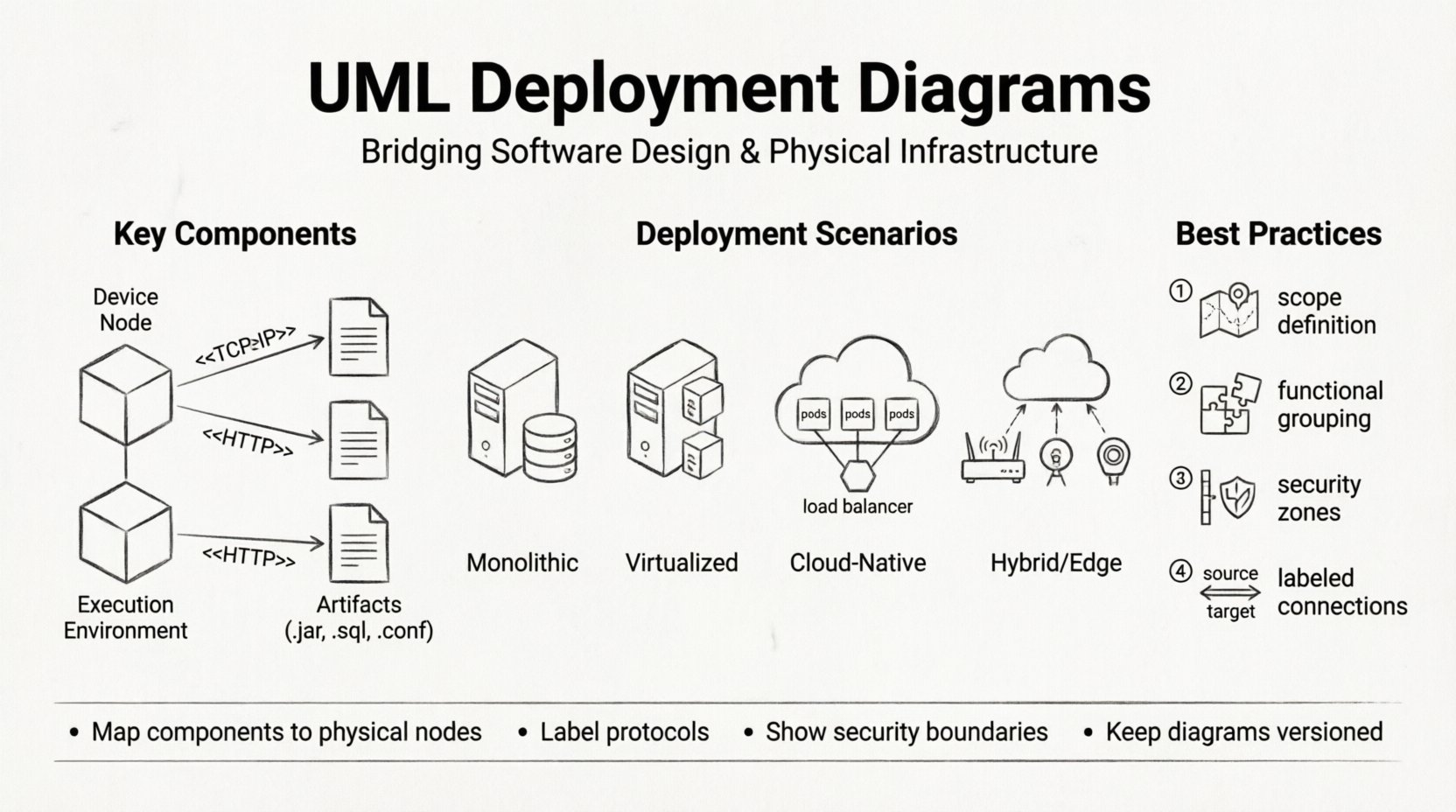
1. Nodes (🖥️)
A node represents a physical or computational resource. It is depicted as a three-dimensional cube. There are two main types:
- Device Nodes: Represent hardware devices such as servers, routers, firewalls, or workstations. These are often the endpoints of communication.
- Execution Environment Nodes: Represent software environments where artifacts are executed, such as an operating system, a virtual machine, or a container runtime.
2. Artifacts (📦)
Artifacts are the physical representations of software components. They are the actual files or executables deployed onto the nodes. Examples include:
- Executable binaries (.exe, .jar)
- Database schemas (.sql)
- Configuration files (.conf)
- Container images (.tar)
Artifacts are shown as documents placed inside or on top of nodes. The relationship between an artifact and a node is typically a composition relationship, implying the artifact resides on the node.
3. Associations and Dependencies (🔗)
Links connect nodes to other nodes or artifacts to nodes. These lines define the flow of data and control.
- Communication Pathways: Represented by solid lines, often with stereotypes like <
> or < > to specify the protocol. - Dependency: Represented by dashed lines, indicating that one node relies on another to function correctly.
- Association: Indicates a structural connection between two elements.
🌍 Real-World Deployment Scenarios
Theoretical knowledge is insufficient without practical application. Below are common scenarios where deployment diagrams provide essential value. Each scenario presents different challenges regarding connectivity, security, and scalability.
Scenario 1: The Traditional On-Premise Monolith
In legacy environments, software often runs on a single physical server or a tightly coupled cluster. The deployment diagram here is relatively simple but requires precision.
- Node Structure: A single Application Server node hosting the Operating System.
- Artifacts: A single WAR file or executable deployed directly to the server.
- Database: A separate Database Server node connected via a secure internal network.
- Communication: JDBC or direct socket connections between the application and database nodes.
This model is straightforward but presents single points of failure. The diagram must clearly show redundancy if high availability is configured, such as dual power supplies or mirrored storage arrays.
Scenario 2: Virtualized Infrastructure
Modern enterprises often move away from bare metal to virtual machines (VMs). This introduces a layer of abstraction between the hardware and the software.
- Node Structure: A physical Host Server containing multiple Virtual Machine Nodes.
- Artifacts: The VM image itself and the guest operating system installed within it.
- Communication: Traffic flows through virtual switches within the host before reaching the physical network.
When modeling this, it is crucial to distinguish between the physical host and the virtual instances. Overlapping responsibilities can confuse capacity planning. The diagram should indicate the hypervisor layer if it is relevant to the security or performance constraints.
Scenario 3: Cloud-Native Microservices
This is the most complex scenario. The system is distributed across multiple cloud regions or availability zones. The deployment diagram must capture the dynamic nature of the infrastructure.
- Node Structure: A Cluster Node representing a managed service (e.g., Kubernetes Cluster). Inside, there are multiple Pod Nodes.
- Artifacts: Container images deployed to the orchestrator.
- Communication: Internal service mesh traffic (e.g., gRPC) and external ingress traffic via a Load Balancer.
- External Dependencies: Connections to managed services like object storage, message queues, or database-as-a-service.
In this context, the diagram acts as a topology map. It helps identify latency issues between regions and ensures that data sovereignty rules are met by showing which nodes reside in which geographic zones.
Scenario 4: Hybrid and Edge Computing
Some systems require processing at the edge (near the data source) while maintaining a central cloud presence.
- Node Structure: Edge Devices (IoT sensors, gateways) connected to a Central Cloud Node.
- Artifacts: Lightweight agents on edge devices, heavy processing logic in the cloud.
- Communication: Asynchronous messaging or batched data transfer to handle intermittent connectivity.
Deployment diagrams for edge computing must highlight network reliability. The diagram should show fallback mechanisms, such as local storage on the edge node if the central connection is lost.
📊 Comparison of Deployment Models
To clarify the differences between these scenarios, consider the following comparison table.
| Feature | Monolithic | Virtualized | Cloud-Native | Edge/Hybrid |
|---|---|---|---|---|
| Primary Node Type | Physical Server | Virtual Machine | Container Cluster | Distributed Devices |
| Deployment Unit | Binary/Archive | ISO/Image | Container Image | Agent/Script |
| Scalability | Vertical (Scale Up) | Vertical/Horizontal | Horizontal (Auto-Scaling) | Distributed Processing |
| Network Dependency | Low (Internal) | Medium (LAN) | High (WAN/Internet) | Variable/Intermittent |
🛠️ Best Practices for Modeling
Creating a deployment diagram is an exercise in abstraction. If the diagram is too detailed, it becomes cluttered. If it is too abstract, it loses utility. Follow these guidelines to maintain clarity.
- Define the Scope: Decide whether you are modeling the entire enterprise infrastructure or a specific application context. Do not mix the two.
- Group by Function: Use compartments to group nodes by function, such as “Web Tier,” “Application Tier,” and “Data Tier.” This helps stakeholders navigate the diagram quickly.
- Use Stereotypes: Leverage standard stereotypes like <
>, < >, < >, and < > to make the diagram universally understandable without excessive text. - Indicate Security Zones: Use dashed lines or shaded areas to represent firewalls, DMZs, and trusted networks. This is critical for security audits.
- Label Connections: Never leave a connection line unlabeled. Specify the protocol (e.g., <
>, < >). This reveals potential bottlenecks or security risks. - Version Control: Treat the diagram as code. Store it alongside the source code repository. Infrastructure changes frequently, and the diagram must reflect the current state.
🚫 Common Pitfalls to Avoid
Even experienced architects can make mistakes when modeling deployment. Be aware of these common issues.
- Over-Engineering: Trying to model every single server in a large organization creates an unreadable mess. Focus on the nodes that run your specific application logic.
- Ignoring Latency: Placing nodes in the diagram without considering their physical distance can lead to performance issues. Indicate geographic locations if relevant.
- Mixing Logical and Physical: Do not put logical component diagrams inside physical nodes. Keep the logical design separate. The deployment diagram is strictly about physical placement.
- Static Representation: Infrastructure is dynamic. A deployment diagram that shows a single node for a load-balanced cluster is misleading. Use the diagram to show the architecture pattern, not necessarily the exact count of instances.
- Missing External Dependencies: It is common to forget third-party services. If your system calls an external API, model that external system as a node or artifact to clarify the boundary.
🔗 Integration with Other Diagrams
A deployment diagram does not exist in isolation. It complements other UML diagrams to provide a complete architectural view.
Component Diagrams
Component diagrams show the logical structure of the software. The deployment diagram maps these components to physical nodes. For example, a Component Diagram might show an “Order Service.” The Deployment Diagram shows that the “Order Service” artifact is deployed to Node “App-Server-01”.
Sequence Diagrams
Sequence diagrams show the flow of messages over time. The Deployment Diagram provides the context for these messages. When a Sequence Diagram shows a message from “Client” to “Server,” the Deployment Diagram confirms that these are distinct physical nodes connected via a network.
Use Case Diagrams
Use Case diagrams describe functionality. They do not show infrastructure. However, the Deployment Diagram helps identify which nodes support which actors. For instance, a “Remote User” actor might connect to a “Firewall Node” before accessing the “Web Server Node”.
🔄 Maintenance and Evolution
Infrastructure evolves. Applications are refactored, servers are retired, and cloud providers change. The deployment diagram must evolve with them. Here is how to keep it relevant.
- Regular Reviews: Schedule quarterly reviews of the deployment diagrams with the operations team. They know the physical reality best.
- Change Management: When a deployment ticket is approved that changes the infrastructure, update the diagram immediately. Do not defer this task.
- Automation: Where possible, generate diagrams from infrastructure as code (IaC) templates. This ensures the diagram is always in sync with the actual configuration.
- Documentation Links: Link the diagram to runbooks and operational guides. If a node fails, the diagram should help locate the documentation for recovery.
🏁 Summary of Value
The deployment diagram is a critical tool for aligning software design with physical reality. It prevents the common disconnect between developers who write code and operations teams who manage servers. By clearly defining nodes, artifacts, and connections, teams can anticipate deployment challenges before they occur.
Whether the system is a simple monolith or a distributed cloud-native application, the principles of modeling remain consistent. Focus on clarity, maintain accuracy, and ensure the diagram serves as a living document rather than a static artifact. This approach ensures that the architecture remains robust, scalable, and understandable throughout the system lifecycle.

